Single Cylinder Solution
First, consider a single unconstrained thick-walled cylinder under pressure loading as shown in
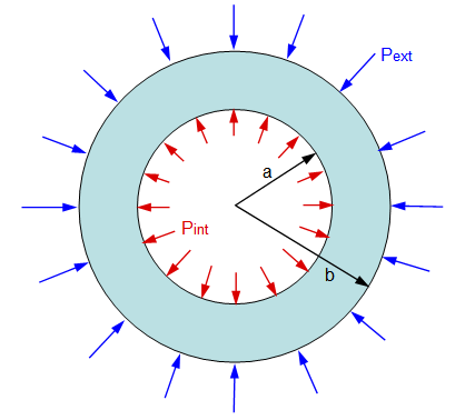
Figure 11 below. The objective is to determine the stresses, strains, and deflections throughout
the cylinder.
Figure 11. Thick-Walled Cylinder Under Internal and External Pressure Loading
The linear solution to this problem is attributed to the French mathematician Gabriel Lame' in
1833. According to his solution, the radial and hoop stresses at any radial location, r, are given by
the following formulas:
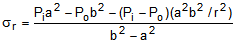 (1a)
(1a)
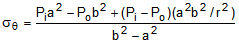 (1b)
(1b)where,
sr = radial stress
sq = hoop stress
r = radius
a = inner radius
b = outer radius
Pi = internal pressure
Po = external pressure
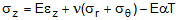
In addition, if the cylinder is fully or partially constrained axially then a uniform axial stress also
develops which is given by,
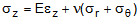 (1c)
(1c)where,
sz = axial stress
E = tensile modulus
n = Poisson ratio
ez = applied axial strain (zero if fully constrained)
If the cylinder is unconstrained then sz = 0 and the induced axial strain is given by,
Eqns. 1a-1c are commonly referred as the Lame' equations and are the foundation for the Concyl
solution algorithm. The derivation of Lame's equations requires the standard application of force
equilibrium equations, linear strain-displacement relations, and isotropic Hookean constitutive
relations, all in polar coordinates. We will make use of the same strain-displacement and
constitutive relations in the Concyl algorithm derivation that follows. The linear strain-
displacement relations in polar coordinates for a generalized plane strain axisymmetric problem
are
 (2a)
(2a) (2b)
(2b) , from generalized plane strain (2c)
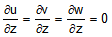 , from generalized plane strain (2d)
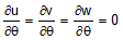 , from axisymmetry (2e)
where,
er = radial strain
eq = hoop strain
ez = axial strain
u = radial deflection
v = hoop deflection
w = axial deflection
r = radial direction
q = hoop direction
z = axial direction
The 3D constitutive relations for an isotropic Hookean material can be expressed as
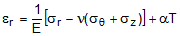 (3a)
(3a)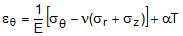 (3b)
(3b)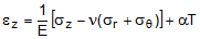 (3c)
(3c)where,
a = coefficient of thermal expansion
T = temperature difference relative to To
To = stress-free temperature
Eqn. (3c) can be rearranged as
 (4)
(4)Substituting Eqn. (3b) into Eqn. (2b) yields the following formula for the radial displacement:
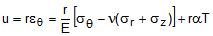 (5)
(5)Substituting Eqn. (4) into Eqn. (5) yields
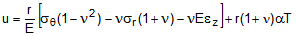 (6)
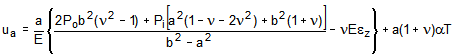
(6)Eqn. (6) gives the radial displacement throughout the cylinder in terms of the radial stress and
hoop stress. The radial and hoop stresses are given by the Lame' equations. Substituting Eqns.
(1a) and (1b) into Eqn. (6) gives the following formulas for the radial displacement at the inner and
outer surfaces of the cylinder.
 (7a)
(7a)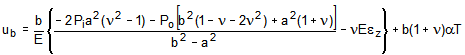 (7b)
(7b)where,
ua = inner radial deflection
ub = outer radial deflection
Multi-Cylinder Solution
Extension of the single cylinder solution to a system of concentric bonded cylinders begins by
enforcing the kinematic compatibility constraint at the interface between each cylinder. The outer
radial deflection of any cylinder must equal the inner radial deflection of the cylinder that is bonded
to its outer surface. This statement leads to the equation
 , i = 1, N-1 (8)
for each pair of bonded cylinders, where i is the cylinder number starting at 1 for the innermost
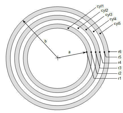
cylinder and ending at N for the outermost cylinder. Figure 12 below shows the cylinder and
interface numbering scheme for a system of five cylinders. Note that the i in Eqn. (8) goes from
1 to N-1 because the inner surface of cylinder 1 is a free surface, as is the outer surface of
cylinder N.
Figure 12. Cylinder and Interface Numbering Scheme
Next, consider a system with only two bonded cylinders. The interfaces will then be numbered
from 1 to 3, and the cylinders numbered from 1 to 2. The i in Eqn. (8) will go from 1 to 1, which
means only a single equation is needed to represent the system. Substituting Eqns. (7a) and (7b)
into Eqn. (8) and collecting like coefficients for the interface pressure terms yields an equation
with the following form:
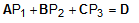 (9)
(9)where the subscripts denote the interface numbers. Since interfaces 1 and 3 are free surfaces,
the values of P1 and P3 are given as input. Therefore, only P2 is unknown, and Eqn. (9) can be
readily solved. The values of A, B, C, and D in the Eqn. (9) are as follows:
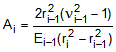 (10a)
(10a)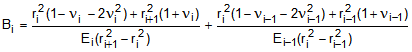 (10b)
(10b)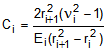 (10c)
(10c) (10d)
(10d)with i ranging from 2 to N, where N is the total number of cylinders. The i subscript on the radius
denotes the radial interface number. The i subscript on the material properties (E,n,a,T)
denotes
the cylinder number. The interfaces and cylinders are numbered in accordance with the
numbering scheme shown in Figure 10.
Extending the solution to an arbitrary number of cylinders results in the following tridiagonal
system of equations with one row for each interface:
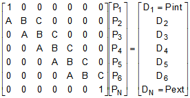 (11)
(11)
The first and last rows have the internal and external pressure boundary conditions. This system
of equations can be readily solved using Gauss elimination to yield all of the unknown interface
pressures between the cylinders. Once these interface pressures are known, then they can be
substituted back into the Lame' equations [Eqn. (1)] to determine the stresses throughout each
cylinder at any arbitrary radius. The stresses can then be used to compute the corresponding
strains using the constitutive relations [Eqn. (3)]. Finally, the radial displacements can computed
from the strains using the strain-displacement relations [Eqn. (2)].
Program Flow
The Concyl solver does the following steps:
1. Read input file
2. Build system equations
3. Solve for unknown interface pressures
4. Compute stresses
5. Compute strains
6. Compute displacements
7. Compute strain energies
8. Write output files
If an optimizer run is requested, then the specified input parameter is varied within the specified
range, and the above steps are repeated to compute the specified solution quantity as a function
of the specified input parameter. If a single optimum value of the input parameter is requested,
then a bisection search is done to find the optimum value. If no optimum solution can be found
within the specified range of input values, then an error message is displayed.
Maximum Shear
The maximum shear stresses and strains are computed from the formulas,
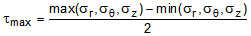 (12a)
(12a) (12b)
(12b)where,
tmax = maximum shear stress
gmax = maximum engineering shear strain
Strain Energy
The strain energy results are computed from the formulas,
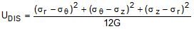 (13a)
(13a)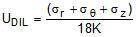 (13b)
(13b)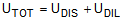 (13c)
(13c)where,
UDIS = distortional strain energy
UDIL = dilatational strain energy
UTOT = total strain energy
G = shear modulus
K = bulk modulus
Equivalent (Von-Mises) Stress
Von-Mises or equivalent stress is commonly used as the yield failure criterion for ductile metals. It
is given by the formula,
 (14)
(14)where,
 = von-mises stress
 = principal stresses (
 )
)Comparison of Eqn. (14) and Eqn. (13a) shows that the von-mises stress is proportional to the
square root of the distortional strain energy [Eqn. (13a)] in accordance with the following relation:
 (15)
(15)Concyl computes von-mises stress and does save it to the output and plot files. However, the
GUI cannot yet display von-mises stress results.