|
2. Thick Pipe Thermal Gradient
|
Previous Next |
Table 2.1. Material Properties
|
Material
|
Designation
(Reference) |
Tensile
Modulus (psi) |
Poisson
Ratio |
CTE
(/°F) |
Ref. Temp.
(°F) |
Density.
(lb/in3) |
|
Steel
|
301 Stainless
(MIL-HDB-5H) |
28e6
|
0.27
|
8.55e-6
|
77
|
0.286
|
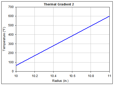
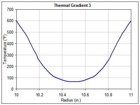
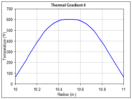
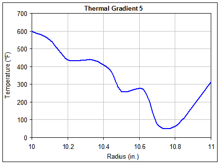
Table 2.2. Loading Requirements
|
Pressure
(psi) |
Temperature
(°F) |
Axial Constraint
|
|
0 to 1000
|
65 to 600
|
Plane Strain (ez = 0)
|
Table 2.3. Load Cases
|
Case
|
Pressure
(psi) |
Temperature
(°F) |
|
1
|
0
|
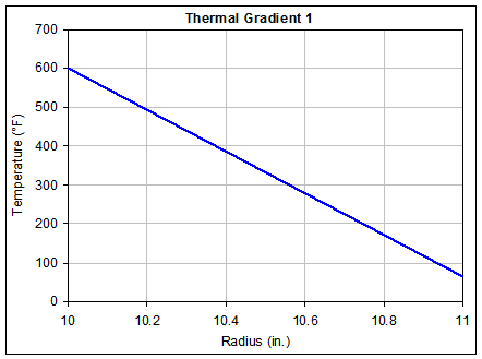
Gradient 1, Fig. 2.1a
|
|
2
|
0
|
Gradient 2, Fig. 2.1b
|
|
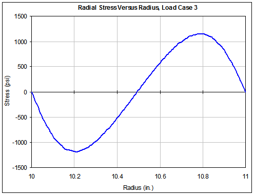
3
|
0
|
Gradient 3, Fig. 2.1c
|
|
4
|
0
|
Gradient 4, Fig. 2.1d
|
|
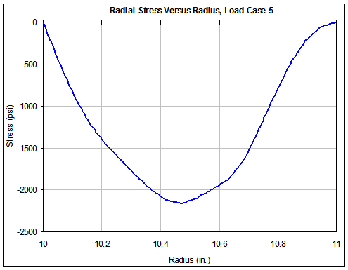
5
|
0
|
Gradient 5, Fig. 2.1e
|
|
6
|
1000
|
Gradient 1, Fig. 2.1a
|
|
7
|
1000
|
Gradient 2, Fig. 2.1b
|
|
8
|
1000
|
Gradient 3, Fig. 2.1c
|
|
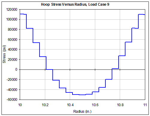
9
|
1000
|
Gradient 4, Fig. 2.1d
|
|
10
|
1000
|
Gradient 5, Fig. 2.1e
|
Table 2.4. Radial Temperature Variation For Each Load Case
|
Radius
|
Case1
|
Case2
|
Case3
|
Case4
|
Case5
|
|
10.00000
|
600.0
|
65.0
|
600.00
|
65.00
|
600.00
|
|
10.05263
|
571.8
|
93.2
|
521.05
|
149.21
|
573.68
|
|
10.10526
|
543.7
|
121.3
|
439.47
|
233.68
|
544.21
|
|
10.15789
|
515.5
|
149.5
|
334.21
|
320.53
|
486.32
|
|
10.21053
|
487.4
|
177.6
|
237.47
|
404.21
|
439.92
|
|
10.26316
|
459.2
|
205.8
|
174.84
|
475.26
|
439.54
|
|
10.31579
|
431.1
|
233.9
|
122.95
|
535.26
|
439.15
|
|
10.36842
|
402.9
|
262.1
|
96.11
|
569.47
|
420.99
|
|
10.42105
|
374.7
|
290.3
|
76.84
|
592.11
|
391.75
|
|
10.47368
|
346.6
|
318.4
|
68.95
|
597.37
|
310.20
|
|
10.52632
|
318.4
|
346.6
|
68.95
|
597.37
|
262.12
|
|
10.57895
|
290.3
|
374.7
|
76.84
|
592.11
|
266.37
|
|
10.63158
|
262.1
|
402.9
|
96.11
|
569.47
|
250.55
|
|
10.68421
|
233.9
|
431.1
|
122.95
|
535.26
|
115.51
|
|
10.73684
|
205.8
|
459.2
|
174.84
|
475.26
|
71.32
|
|
10.78947
|
177.6
|
487.4
|
237.47
|
404.21
|
66.05
|
|
10.84211
|
149.5
|
515.5
|
334.21
|
320.53
|
113.42
|
|
10.89474
|
121.3
|
543.7
|
439.47
|
233.68
|
173.95
|
|
10.94737
|
93.2
|
571.8
|
521.05
|
149.21
|
246.32
|
|
11.00000
|
65.0
|
600.0
|
600.00
|
65.00
|
320.00
|
Table 2.5. Applied Cylinder Delta Temperature For Each Load Case
|
Cyl
|
DT1
|
DT2
|
DT3
|
DT4
|
DT5
|
|
1
|
508.921
|
2.079
|
483.526
|
30.105
|
509.842
|
|
2
|
480.763
|
30.237
|
403.263
|
114.447
|
481.947
|
|
3
|
452.605
|
58.395
|
309.842
|
200.105
|
438.263
|
|
4
|
424.447
|
86.553
|
208.842
|
285.368
|
386.119
|
|
5
|
396.289
|
114.711
|
129.158
|
362.737
|
362.729
|
|
6
|
368.132
|
142.868
|
71.895
|
428.263
|
362.342
|
|
7
|
339.974
|
171.026
|
32.526
|
475.368
|
353.068
|
|
8
|
311.816
|
199.184
|
9.474
|
503.789
|
329.368
|
|
9
|
283.658
|
227.342
|
-4.105
|
517.737
|
273.975
|
|
10
|
255.500
|
255.500
|
-8.053
|
520.368
|
209.162
|
|
11
|
227.342
|
283.658
|
-4.105
|
517.737
|
187.244
|
|
12
|
199.184
|
311.816
|
9.474
|
503.789
|
181.460
|
|
13
|
171.026
|
339.974
|
32.526
|
475.368
|
106.033
|
|
14
|
142.868
|
368.132
|
71.895
|
428.263
|
16.414
|
|
15
|
114.711
|
396.289
|
129.158
|
362.737
|
-8.316
|
|
16
|
86.553
|
424.447
|
208.842
|
285.368
|
12.737
|
|
17
|
58.395
|
452.605
|
309.842
|
200.105
|
66.684
|
|
18
|
30.237
|
480.763
|
403.263
|
114.447
|
133.132
|
|
19
|
2.079
|
508.921
|
483.526
|
30.105
|
206.158
|
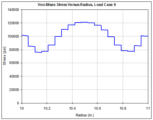
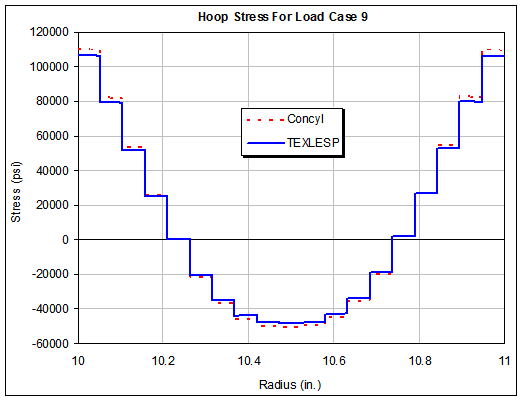
Table 2.6. Concyl Stress Results
|
Case
|
Loading
|
Tensile Stress
(ksi)
|
Von-Mises Stress
(ksi)
|
|
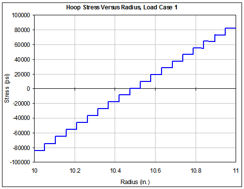
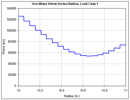
1
|
|
81.8 H (o)
|
125.8 (i)
|
|
2
|
|
84.5 H (i)
|
125.0 (o)
|
|
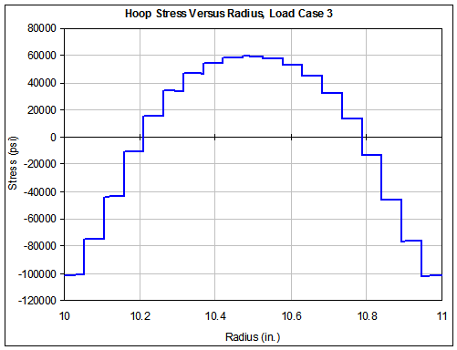
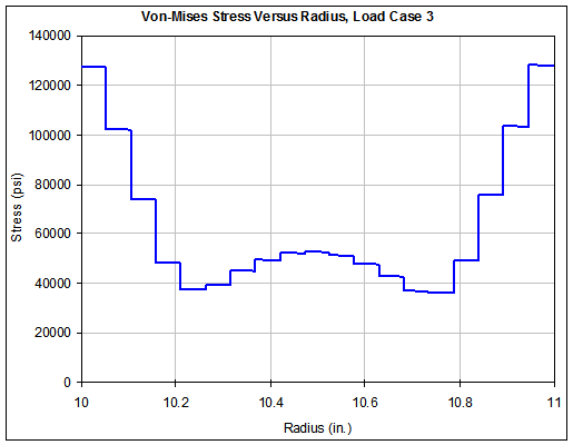
3
|
|
84.5 H (m)
|
127.7 (i,o)
|
|
4
|
|
99.8 H (i,o)
|
122.4 (m)
|
|
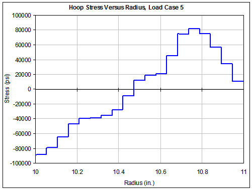
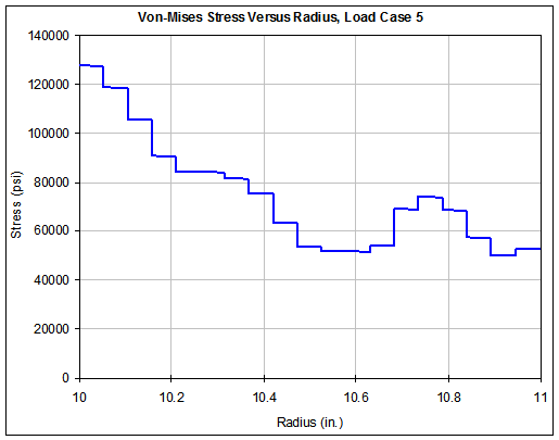
5
|
|
82.2 H (m)
|
127.3 (i)
|
|
6
|
|
91.6 H (o)
|
122.1 (i)
|
|
7
|
|
95.0 H (i)
|
122.4 (o)
|
|
8
|
|
69.4 H (m)
|
123.8 (i,o)
|
|
9
|
|
110.5 H (i,o)
|
121.0 (m)
|
|
10
|
|
91.9 H (m)
|
123.5 (i)
|
|
|
Variability
|
45%
|
5%
|
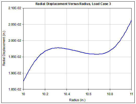
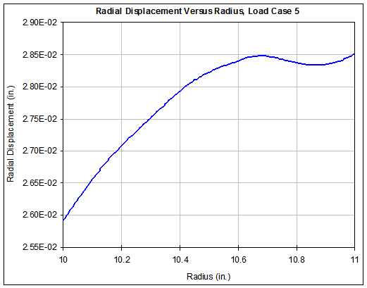
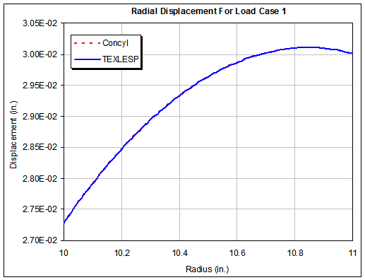
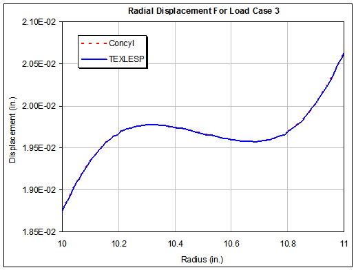
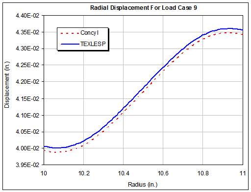
Table 2.7. Concyl Displacement Results
|
Case
|
Loading
|
Inner (E-2 in.)
|
Outer (E-2 in.)
|
|
1
|
|
2.73
|
3.00
|
|
2
|
|
2.82
|
3.10
|
|
3
|
|
1.88
|
2.06
|
|
4
|
|
3.63
|
4.00
|
|
5
|
|
2.59
|
2.85
|
|
6
|
|
3.10
|
3.35
|
|
7
|
|
3.18
|
3.45
|
|
8
|
|
2.24
|
2.41
|
|
9
|
|
3.99
|
4.34
|
|
10
|
|
2.96
|
3.20
|
|
|
Variability
|
72%
|
71%
|
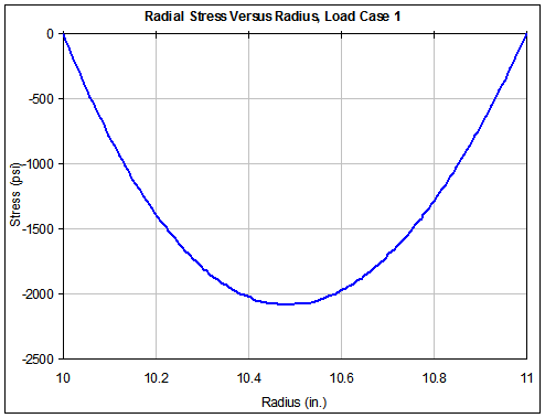
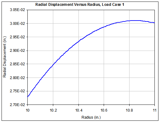
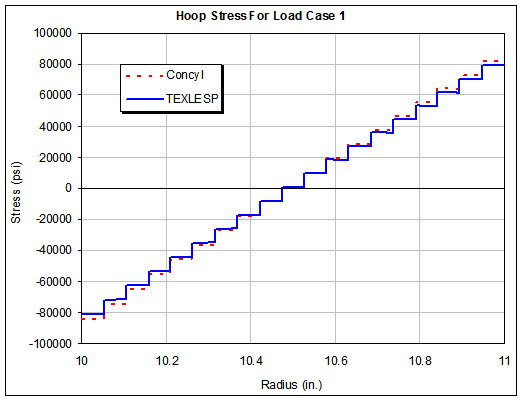
Concyl Load Case 1 Listing
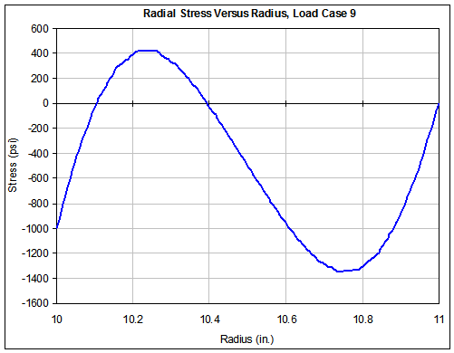
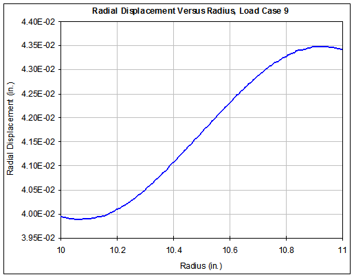
TEXLESP Load Case 9 Listing