1. Shrink-Fit Pipe

1. Shrink-Fit Pipe Under Thermal And Pressure Loading

Previous Next

1.1. Problem Description

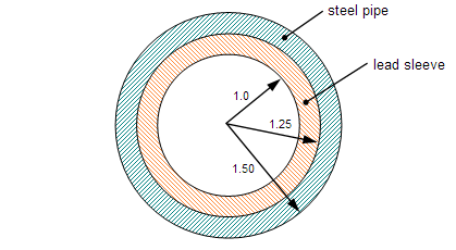
Consider a long thick-walled pipe with two material layers as shown in Figure 1.1. The inner layer is made of lead with an inner radius 1.00 in. and an outer radius of 1.25 in. at a temperature of 77°F. The outer layer is steel with an inner radius of 1.25 in. and an outer radius of 1.50 in. at a temperature of 250°F. The two layers are joined by a shrink-fit once the outer layer has cooled to the same temperature as the inner layer.

The pipe assembly is designed to carry a radioactive fluid over a range of pressures and temperatures. Figure 1.1 shows the pipe cross section dimensions prior to the shrink-fit assembly. Table 1.1 lists the material properties for each layer, and Table 1.2 gives the loading requirements. The thermal loading is uniform with no temperature variation through the pipe thickness. Also, the pipe is fully constrained axially so that the axial strain is zero.

Figure 1.1. Dual-Layer Pipe Geometry (Stress Free)

Table 1.1 Material Properties

Material	Designation (Reference)	Tensile Modulus (psi)	Poisson Ratio	CTE (/°F)	Ref. Temp. (°F)	Density. (lb/in³)
Lead	Lead (wikipedia.com)	2.32e6	0.44	1.61e-5	77	0.410
Steel	301 Stainless (MIL-HDBK-5H)	28e6	0.27	8.55e-6	250	0.286

Table 1.2. Loading Requirements

Pressure (psi)	Temperature (°F)	Axial Constraint
100 to 1000	-25 to 200	Full (ez = 0)

1.2. Objectives

1. Use Concyl to determine the following:

a. The initial radial overlap between the pipe layers at room temperature (77°F) prior to assembly.

b. The interface pressure between the pipe layers at room temperature after assembly (thermal loading only).

c. The maximum tensile stresses and strains in each layer at the upper and lower pressure and temperature limits.

d. The critical low temperature for layer separation at the lower and upper pressure limits.

2. Use finite-element analysis (FEA) to verify the Concyl results.

1.3. Key Assumptions

1. Linear, elastic, and isotropic materials

2. Linear kinematics

3. Uniform thermal loading (no temperature variation in any direction)

4. Plane strain in axial direction

5. Perfectly bonded cylinders (no sliding at interfaces)

1.4. Concyl Analysis

Concyl can readily meet all four of the above objectives (1a through 1d). The first objective, however, can be answered using elementary formulas without the use of any numerical tools. The remaining objectives are a little more difficult and do require either an exact numerical tool such as Concyl or an approximate numerical approach, such as the finite element method.

Five load cases were analyzed here to consider all the possible permutations of applied temperature and pressure in accordance with the loading requirements listed in Table 1.2. Load case 1 gives the results needed to satisfy objectives 1a and 1b. The other load cases provide the results needed determine the overall peak stresses and strains for objective 1c. Objective 1d was answered using the Concyl optimizer to determine the critical temperature for a zero interface pressure between the cylinders at the upper and lower pressure limits.

Table 1.3. Load Cases

Case	Pressure (psi)	Temperature (°F)
1	0	77
2	100	-25
3	1000	-25
4	100	200
5	1000	200

1.4.1. Radial Overlap

The first objective for this problem is to determine the radial interference between the layers at room temperature. This can be readily done using the dimensions in Figure 1.1 and the material properties in Table 1.1 together with some basic formulas. For small strains and small rotations the hoop strain is related to the radial deformation by the equation,

(1.1)

where,

e_h= hoop strain

Dr = radial growth (Dr = r_f- r)

r_f = final radius

r = initial radius (stress-free)

For a linear isotropic material the strain induced by thermal loading is equal in all directions and is given by,

(1.2)

where,

a= coefficient of thermal expansion (CTE)

DT= temperature relative to the stress-free temperature (DT = T - T₀)

T = applied temperature

T₀ = stress-free temperature

Combining Eqns. 1.1 and 1.2 yields the following formula for the radial growth within each layer as a function of temperature:

(1.3)

Considering a temperature of 77°F and using the values from Figure 1.1 and Table 1.1, the following values of Dr at the interface are computed:

Inner Layer: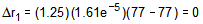

Outer Layer: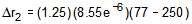

= -0.00185

Since the inner layer reference temperature is 77 F, the induced thermal strain is zero which means no radial growth. The radial gap between the layers is then given by

= -0.00185 ¬¾¾ Radial Overlap at 77°F (1.4)

where a positive value denotes a gap and a negative value denotes an interference. In this case we have a radial overlap at room temperature that is slightly less than 2 mils. That is how much the inner radius of the steel layer would decrease (stress free) if it were to cool to 77°F in the absence of the inner layer. However, the presence of the inner layer will result in a contact pressure between the two layers as the outer layer shrinks against the inner layer. This contact pressure joins the layers together and induces stresses in each layer.

1.4.2. Interface Pressure

The Concyl results for load case 1 give the interface pressure between the layers at room temperature. The Concly input and output for load case 1 are provided in Listing 1.1a and Listing 1.1b at the end of this report. Concyl computes an interface pressure of 1247 psi for the unpressurized pipe at 77°F.

1.4.3. Maximum Stresses and Strains

The Concyl results for load cases 2 through 5 give the stresses and strains in each layer under the required operational pressure and temperature limits. Table 1.4 lists the maximum tensile hoop stresses and strains in each layer along with the interface pressure (radial stress) for each load case. The maximum stress location within each layer is also indicated by an I (inner) or O (outer). This table shows that the lead layer remains in compression with a negative hoop strain for all load cases. The steel layer remains in tension for all load cases, even though the corresponding hoop strains are negative for load cases 1 through 3.

Table 1.4. Concyl Stress and Strain Results

Hoop Stress / Strain (psi / %)

Case	Interface Pressure (psi)	Inner Layer	Outer Layer
1	1247	-5682 / -0.1634 (O)	6916 / -0.0155 (I)
2	494	-1897 / -0.1247 (O)	2742 / -0.0538 (I)
3	1233	-2061 / -0.1102 (O)	6838 / -0.0393 (I)
4	2336	-10.28e3 / -0.2066 (O)	12.95e3 / 0.0342 (I)
5	3074	-10.45e3 / -0.1921 (O)	17.05e3 / 0.0487 (I)

The maximum tensile stress that occurs throughout the required pressure and temperature ranges is 17.05 ksi, and the corresponding maximum strain is 0.0487%. These both occur at the inner surface of the steel layer for load case 5. Table 1.5 gives a summary of the pipe stress analysis results computed from Concyl.

Table 1.5. Concyl Result Summary

Condition	Value	Load Case	Temp. (°F)	Press. (psi)
Min. Interface Pressure	464	2	-25	100
Max. Interface Pressure	3074	5	200	1000
Max. Tensile Stress	17.05e3	5	200	1000
Max. Tensile Strain	0.0487	5	200	1000

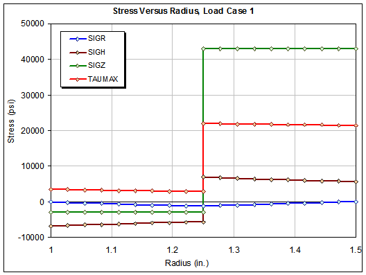
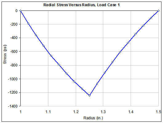
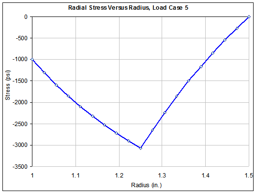
Figure 1.2 shows a plot of the four stress components versus radius for load case 1. Note that all of the stress components, except for the radial stress, have a step discontinuity at the material interface. This is to be expected since each layer is a different material, and the induced stresses for this load case are highly dependent on the material properties. However, the plot of radial stress, which is shown in Figure 1.3, must be continuous, and the radial stress value at the layer interface must be equal in both materials to enforce static equilibrium. The first derivative in Figure 1.3 is discontinuous, as expected, and shows the peak compressive interface pressure of 1247 psi which agrees with the value listed in Table 1.4.

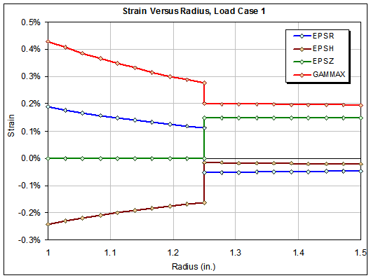
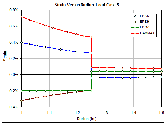
Figure 1.4 shows how the radial strain varies with radius. All four of the strain components have step discontinuities. This means that the first derivative of the strain with respect to radius is infinite at the material interface. This is to be expected when thermal loading is applied since these strain values are mechanical strains, not total strains.

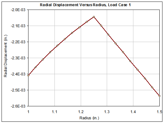
Figure 1.5 shows the radial displacement variation through the pipe. This plot must be continuous to enforce displacement compatibility at the interface. If it were discontinuous, then a crack or overlap at the interface would be indicated. The radial displacement is negative throughout the pipe. This is expected since the applied thermal strain is negative and there is no internal pressure loading.

Figure 1.2. Stress Versus Radius For Load Case 1

Figure 1.3. Radial Stress Versus Radius For Load Case 1

Figure 1.4. Strain Versus Radius For Load Case 1

Figure 1.5. Radial Displacement Versus Radius For Load Case 1

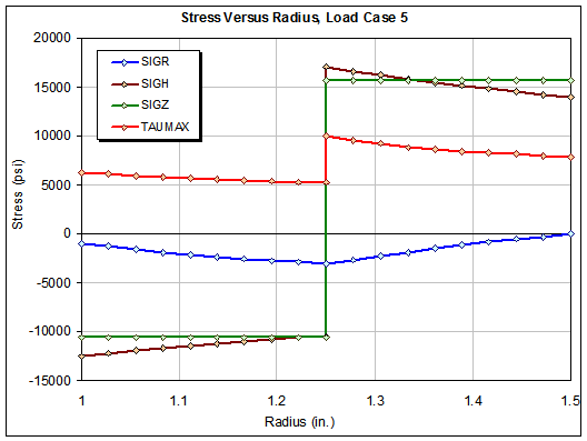
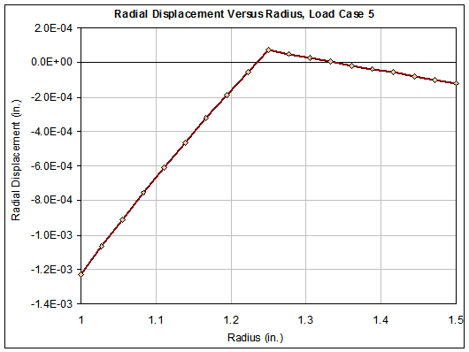
Figures 1.6 through 1.9 show plots of the Concyl results for load case 5. This load case has a 200°F thermal load combined with a 1000 psi internal pressure load. These plots show that the steel layer carries all the tension load from the applied pressure, while the inner lead layer remains in compression. The results also show that the inner layer has much greater strain magnitudes because of the softer lead. Figure 1.9 shows that for this particular load case, positive radial displacement is predicted near the material interface, but the radial displacement is negative elsewhere.

Figure 1.6. Stress Versus Radius For Load Case 5

Figure 1.7. Radial Stress Versus Radius For Load Case 5

Figure 1.8. Strain Versus Radius For Load Case 5

Figure 1.9. Radial Displacement Versus Radius For Load Case 5

1.4.4. Critical Temperature

Determining the critical low temperature that would cause a loss of compression between the layers was very straightforward using the Concyl optimizer. The applied temperature was specified as the input parameter, and the radial stress between the cylinders was specified as the output parameter. The desired optimum value for the radial stress was entered as zero. The lower and upper limits for the temperature search range were specified as -200°F and 0°F respectively. One optimization run was done at the low pressure limit of 100 psi, and another run was done at the high pressure limit of 1000 psi. The Concyl optimization input file for the low pressure run is shown in Listing 1.2. 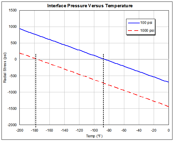Table 1.6 gives the results from the optimization runs. Figure 1.10 shows a plot of the interface pressure as a function of temperature at operational pressure of 100 psi and 1000 psi.

Table 1.6 Concyl Optimizer Results

Pressure	Critical Temperature (°F)
100	-85.4
1000	-175.7

Figure 1.10. Interface Pressure Versus Temperature

1.5. Finite Element Analysis

Confirmation of the Concyl results was done with two different FEA programs: NISA and TEXLESP2D. NISA is a commercial general purpose FEA program that is described in Ref. 1. TEXLESP2D is a specialized NASA program developed for nonlinear 2D stress analysis (Ref. 2). A single finite element model was made for use with both programs. Five runs were done to analyze the load cases listed in Table 1.3. In addition, another set of runs was done to verify the critical temperature calculations that were done by the Concyl optimizer. This gives two more load cases with the loads listed in Table 1.6. Load case 6 has an applied pressure of 100 psi, and load case 7 has an applied pressure of 1000 psi.

1.5.1. Model Description

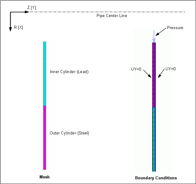
The FEA stress analysis was done with the small 2D model shown in Figure 1.11. The model is axisymmetric with 100 quadratic isoparametric elements. Since this problem has no axial stress variation, only one element is required in the axial direction. Figure 1.11 shows the finite element mesh with each material a different color. Each cylinder has 50 equally spaced elements in the radial direction. This figure also shows the applied pressure and displacement boundary conditions (BC's).

The NISA and TEXLESP2D programs differ in the way that thermal loading is applied to the model. NISA has a single stress-free temperature for the entire model, and temperature BC's are applied to the nodes. TEXLESP2D assigns a stress-free temperature to each material, and a uniform temperature is applied to the entire model. Listing 1.3 at the end of this report shows the NISA input file for load case 5, and Listing 1.4 shows the corresponding TEXLESP2D input file.

Figure 1.11. Finite Element Mesh and Boundary Conditions

1.5.2. NISA Results

Table 1.7 shows the NISA interface pressures for all the load cases. These values are in close agreement with the exact Concyl results listed in Table 1.4. The maximum error in the NISA results is less then 3% which is generally very good for a finite element model. Also, the interface pressures for load cases 6 and 7 are very close to zero as expected.

Table 1.7. NISA Interface Pressure Results

Case	Interface Pressure (psi)	Error (%)
1	1228	-1.52
2	482	-2.43
3	1217	-1.29
4	2321	-0.642
5	3026	-1.56
6	3.47	small
7	3.95	small

1.5.3. TEXLESP Results

Table 1.8 shows the TEXLESP interface pressures for all the load cases. These values are in close agreement with the exact Concyl results listed in Table 1.4. The maximum error in the TEXLESP results is less then 1%. Also, the interface pressures for load cases 6 and 7 are very close to zero as expected. These results show that for this particular problem TEXLESP has less error than NISA.

Table 1.8. TEXLESP Interface Pressure Results

Case	Interface Pressure (psi)	Error (%)
1	1241	-0.481
2	492	-0.405
3	1227	-0.487
4	2325	-0.471
5	3060	-0.455
6	0.293	small
7	0.194	small

1.6. Conclusions

This example demonstrates how to use Concyl to analyze a shrink-fit compound cylinder problem involving combined thermal and pressure loading. Use of the Concyl optimizer was also demonstrated. The Concyl results have good agreement with the results from two separate FEA programs. This verifies that Concyl is an accurate and efficient tool for compound cylinder stress analysis.

References

1. "NISA Users Manual", Engineering Mechanics Research Corporation, 1998. (www.nisasoftware.com)

2. "TEXLESP-2D Users Manual", Eric B. Becker, et al, NASA MSFC-RPT-1564, 1988.

Concyl Listings

Listing 1.1a. Concyl Input For Load Case 1

!Concyl Input File

Load Case 1: P=0, T=77

1, 1.25, 1.5

1, 77

2, 250

1, Lead, 2.32e+006, 0.44, 1.61e-005, 0.41

2, Steel, 2.8e+007, 0.27, 8.55e-006, 0.286

0, 0

ALL

Listing 1.1b. Concyl Output For Load Case 1

------------------------------------------------------

Output Data

------------------------------------------------------

---------------------

Interface Pressures

---------------------

Interface Radius Pressure

--------- ------ --------

1 1.0000 +0.00000

2 1.2500 +1247.2

3 1.5000 +0.00000

Note: Negative pressure means tension

-----------------------------

Cylinder Interface Stresses

-----------------------------

Cyl<Int> SIGH SIGR SIGZ TAUMAX SIGE

-------- ---- ---- ---- ------ ----

1I -6928.8 +0.00000 -3048.7 +3464.4 +6014.9

1O -5681.6 -1247.2 -3048.7 +2840.8 +3862.8

--------------------------------------------------------------------------------

2I +6916.2 -1247.2 +42947. +22097. +40731.

2O +5669.0 +0.00000 +42947. +21473. +40412.

--------------------------------------------------------------------------------

-----------------------------------------

Cylinder Interface Strains (Mechanical)

-----------------------------------------

Cyl<Int> EPSH EPSR EPSZ GAMMAX EPSE

-------- ---- ---- ---- ------ ----

1I -0.0024084 +0.0018923 +0.00000 +0.0043006 +3048.7

1O -0.0016342 +0.0011182 +0.00000 +0.0027524 +3048.7

--------------------------------------------------------------------------------

2I -0.00015510 -0.00052536 +0.0014791 +0.0020045 +42947.

2O -0.00021166 -0.00046880 +0.0014791 +0.0019479 +42947.

--------------------------------------------------------------------------------

------------------------------------

Cylinder Interface Strains (Total)

------------------------------------

Cyl<Int> EPSHT EPSRT EPSZT GAMMAX

-------- ----- ----- ----- ------

1I -0.0024084 +0.0018923 +0.00000 +0.0043006

1O -0.0016342 +0.0011182 +0.00000 +0.0027524

------------------------------------------------------------------

2I -0.0016342 -0.0020045 +0.00000 +0.0020045

2O -0.0016908 -0.0019479 +0.00000 +0.0019479

------------------------------------------------------------------

------------------------------------

Cylinder Interface Strain Energies

------------------------------------

Cyl<Int> Distortion Dilatation Total

-------- ---------- ---------- -----

1I +7.4854 +0.85819 +8.3436

1O +3.0871 +0.85819 +3.9453

------------------------------------------------

2I +25.082 +6.4715 +31.554

2O +24.691 +6.4715 +31.162

------------------------------------------------

-------------------------

Interface Displacements

-------------------------

Interface Radius DispR

--------- ------ -----

1 1.0000 -0.0024084

2 1.2500 -0.0020428

3 1.5000 -0.0025362

Listing 1.2. Concyl Input For Optimization Run

!Concyl Input File

Optimization Run: Invar=Temp, OutVar=SIGR, P=100

1, 1.25, 1.5

1, 77

2, 250

1, Lead, 2.32e+006, 0.44, 1.61e-005, 0.41

2, Steel, 2.8e+007, 0.27, 8.55e-006, 0.286

100, 0

ALL

-200, 0

Listing 1.3. NISA Input For Load Case 5

***********************************************************************

*** CONCYL SAMPLE 1:

*** Compound Cylinder Under Thermal and Pressure Load

***********************************************************************

ANALYSIS = STATIC

SOLVER = FRONTAL

NODE = OFF

ELEMENT = OFF

FILE = result

SAVE = 26,27

SORT = 20

*TITLE

Concyl Sample 1

Compound Cylinder Under Thermal and Pressure Loading

*ELTYPE

1, 3, 2

*NODES

1,,,, 1.00000E+00, 0.00000E+00, 0.00000E+00, 0

2,,,, 1.00500E+00, 0.00000E+00, 0.00000E+00, 0

...

502,,,, 1.49500E+00, 5.00000E-03, 0.00000E+00, 0

503,,,, 1.50000E+00, 5.00000E-03, 0.00000E+00, 0

*ELEMENTS

1, 100, 1, 1, 0

1, 103, 2, 204, 53, 153, 52, 203,

...

100, 200, 1, 1, 0

302, 403, 303, 503, 353, 453, 352, 502,

*MATERIAL

***--------------------------------------------------------------------------

*** Inner Layer, Lead

***--------------------------------------------------------------------------

EX , 100,0, 2.32e6

NUXY, 100,0, 0.44

DENS, 100,0, 0.410

ALPX, 100,0, 1.61e-5

***--------------------------------------------------------------------------

*** Outer Layer, 301 Stainless Steel

***--------------------------------------------------------------------------

EX , 200,0, 27e6

NUXY, 200,0, 0.27

DENS, 200,0, 0.286

ALPX, 200,0, 8.55e-6

*SETS

***--------------------------------------------------------------------------

*** node sets for stress/strain recovery

***--------------------------------------------------------------------------

100,S, 1, 52, 203,

200,S, 51, 102, 253,

300,S, 303, 353, 503,

***--------------------------------------------------------------------------

*** elements sets for stress/strain recovery

***--------------------------------------------------------------------------

400,S, 1, 50, 51, 100

***--------------------------------------------------------------------------

*** load case 1: thermal load at 77 degrees with no pressure

***--------------------------------------------------------------------------

*LDCASE, ID= 1

1, 1, 7, 1, 4, 4, 1, 77.0, .000

*LCTITLE

Temperature = 77, Pressure = 0

*ECHO = OFF

*SPDISP

***--------------------------------------------------------------------------

*** plane strain axial constraints

***--------------------------------------------------------------------------

** SPDISP SET = 1

1,UY , 0.00

2,UY , 0.00

...

453,UY , 0.00

***============================================================================

*** applied pressure load, min = 100, max = 1000

***============================================================================

***PRESSURE

** PRESSURE SET = 1

** 1,,,4,0, 0, 1000, 0

***============================================================================

*** applied thermal load at 77F, min = -25, max = 200

***============================================================================

*NDTEMPER

***----------------------------------------------------------------------------

*** set 1 is the applied temperature to the inner layer

*** which has a stress free temperature of 77F

***----------------------------------------------------------------------------

** NDTEMPER SET = 1

1,TEMP,77.0

2,TEMP,77.0

...

102,TEMP,77.0

51,TEMP,77.0

***----------------------------------------------------------------------------

*** set 3 is the applied temperature to the outer layer

*** which has a stress free temperature of 250F

***----------------------------------------------------------------------------

** NDTEMPER SET = 2

253,TEMP,-96.0

254,TEMP,-96.0

...

502,TEMP,-96.0

503,TEMP,-96.0

*ECHO = ON

*PRINTCNTL, ID=100

AVND,100,200,300

DISP,100,200,300

ELFO,-1

SLFO,-1

RLFO,-1

ELSE,-1

ELST,400

REAC,-1

LDVE,-1

VELO,-1

ACCE,-1

*POSTCNTL, ID=100

NDSTRS, 0

NDSTRN, 0

GPSTRS,-1

NDSTNP,-1

NDSTNC,-1

ERRIND,-1

*ENDDATA

Listing 1.4. TEXLESP2D Input For Load Case 5

$ Concyl Sample 1 Test Case

$------------------------------------------------

$ Plane Strain Compound Cylinder

$ English Units: in,lb,sec,psi

$ Load Case 5

$ Thermal Plus Pressure Loading, T=200, P=1000

$------------------------------------------------

$ Exact Solution:

$ Interface Perssure = 3074 psi

$------------------------------------------------

axisym

thermal,200

$------------------------------------------------

$ material definition

$------------------------------------------------

setup,2,ij,201

iso,lead, 1, 2.32e6, 0.44, 1.61e-5, 77

iso,steel, 2, 27e6, 0.27, 8.55e-6, 250

end,material

$ mesh definition

1,1, 101,3

1.00,1.25,1.25,1.00

0.00,0.00,0.01,0.01

101,1, 201,3

1.25,1.50,1.50,1.25

0.00,0.00,0.01,0.01

end,grid

$------------------------------------------------

$ element definitions

$------------------------------------------------

iloop,50

qq,,1, 1,1

qq,,2, 101,1

iend

$------------------------------------------------

$ boundary conditions

$------------------------------------------------

iloop,100

bc,uy, 1,1, 1

bc,uy, 1,1, 3

iend

bc,pressure, 1,1, 4, 1000.0

end,elements

$------------------------------------------------

$ linear solver

$------------------------------------------------

solve

$------------------------------------------------

$ post processing

$------------------------------------------------

stress

option,linear,15,,,,,1,1,3,3

option,linear,15,,,,,99,1,101,3

option,linear,15,,,,,199,1,201,3

end,stress

stop